
Space Station Cost Simulation Version 0.5, 05/29/2026
Space Station Simulation Documentation Version 0.5, 05/29/2026
User Guide Table of Contents
If you already have experience at using the CSSS Space Station Cost Simulator, you can start the simulation now. If this is your first time here, it is strongly suggested that you read this User Guide first before launching the simulation.
Introduction
Welcome to the CSSS Space Station Design Cost Simulator. This is your opportunity to try your hand at designing a commercial space station within the constraints set by the simulator. This User Guide is the primary documentation for the operation of the simulation and understanding the inputs and outputs.
Your role in the simulation is that of a design manager for a commercial space station company. You have been tasked with the challenge of designing a space station that can be reasonably certain of being economically sustainable, which means that your space station will make sufficient profits so as to recover all capital expenditures and operating expenses associated with the project over the course of its life. You should think of your space station as a system – that is as a set of interrelated components that interact with one another in an organized fashion to achieve a common purpose.
As you experiment with different configurations, you will gain experience with the process of decision analysis because what you are doing is conducting a techno-economic analysis.
Space Station Design as a Techo-Economic Analysis
A techno-economic analysis, or TEA, is a methodology used for evaluating the economic performance of a technology. As a designer, you must weigh the benefits against the costs. In the context of designing a commercial space station, the commercial component means that the design is no longer just an engineering exercise, but is now also a financial exercise. You must design a space station that can deliver goods and services to market at a price that your customer pool is willing to pay. The question is can you do it?
As a part of your analysis, some of the key financial concepts that you may want to familiarize yourself with are:
Capital Expenditures (CapEx)
Operating Expenditures (OpEx)
Net Present Value (NPV)
Internal Rate of Return (IRR)
Weighted Average Cost of Capital (WACC)
This simulation is not just about designing a space station but is about designing a business model that leads to a successful space station enterprise.
Software and Documentation Strategy
The space station simulator software and associated documentation are based on a strategy of continuous design and deployment. Incremental changes may be made to both the software and the documentation.
Space Station Design Overview
To design a commercial space station is an exceedingly complex operation, both technically and financially. Consider for a moment the array of components and systems that a space station is composed of – with every system being linked to and compatible with every other system. The Space Station Structural Components outline below provides an overview of the types of components and systems that one might expect to find as being a part of a space station.
Space Station Structural Components
Pressurized Modules
Habitation Module
Laboratory Module
Manufacturing Module
Logistics/Storage Module
Observation / Recreation Module (Tourism)
Nodes
Module Nodes
Docking Adapters
Truss Structure
External Components
Solar Arrays
Thermal Radiators
External Payloads
Robotic Manipulators
Mobile Transporter Rails
Micrometeoroid and Orbital Debris (MMOD) Protection
Space Station Core Systems
Environmental Control and Life Support System (ECLSS)
Electrical Power System (EPS)
Thermal Control System (TCS)
Attitude and Orbit Control System (AOCS) / Motion Control System (MCS)
Command and Data Handling (C&DH) / Data Management System
Communications and Tracking (C&T) System
Crew and Mission Support Systems
Crew Health Care System (CHeCS)
Robotic Manipulator Systems
Extravehicular Mobility Units (EMU)
The CSSS simulator offers a greatly simplified design scenario to expedite the exploration process. Even though designed as a minimalistic simulation, the simulator models multiple aspects of a space station project. These include:
Development, Design, Test, and Evaluation (DDT&E) costs
Manufacturing learning curves using Wright’s Law
Launch expenditures
Annual operating expenditures (OpEx)
Revenue uncertainty
Discounted future cash flows
Investment risk
Capacity utilization effects
In the modeling of the commercial space station, the program by necessity incorporates a number of major domains:
Orbital mechanics
Atmospheric drag and reboost requirements
Power generation systems
Thermal radiator sizing
Module manufacturing economics
Launch vehicle constraints
Consumables logistics
Tourism revenue
Research revenue
Operational expenditures
Discounted cash flow finance
Net Present Value (NPV)
Internal Rate of Return (IRR)
Monte Carlo risk modeling
Optimization analysis
Insight into some aspects of these domains can be gained by reading through the Relevant System Configuration Constantssection.
In addition to being technically complex, a commercial space station is also financially complex.
Commercial space stations have a serious cost problem which is inextricably linked to the market for goods and services a space station provides. If goods and services produced aboard space stations are to have a positive economic impact, then the issue of design, development, deployment, and operations costs will have to be different from those that have governed the design of government-owned space stations where cost is secondary.
As a part of your exploration of space station design, you will need to be aware of the design trade-offs that must be made and how these trade-offs will impact cost, revenue and ultimately profitability – with profit being the proxy for sustainability.
The left sidebar contains all the user definable inputs and is organized into five sections. Changing any value immediately causes the program to recalculate the entire model and re-render the dashboard. This instant feedback is done so that you can see the impact of any change you make to the design.
Running the Simulation
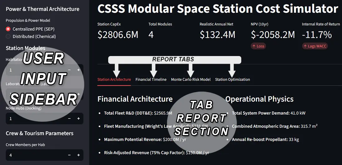
Image 1: The Space Station Design Cost Simulator Web App Main Screen Section Layout
Above you see the default display of the simulator web app as it appears on a large screen. The simulation is divided into four sections. The top-most center panel displays the web app’s name and shows a five-metric summary row of key financial values. Below this is the Report Tabs Selector Row from which one of four detailed report data can be shown in the Tab Report Section that is at the bottom of the main screen. The left side of the program screen contains the User Input Sidebar which you will use to set the values to be used for each run of the simulation. A PDF report download button is located at the bottom of the sidebar. Because of the vertical size of the sidebar, you will need to scroll vertically in order to see all the user input options.
Before proceeding to run the simulation, it is important to note the following items.
1) Program Spin-up
When you first access the web page hosting the simulator, it may take a few minutes for the application to start on the server. When the application is starting, you will see a black screen similar to the following:
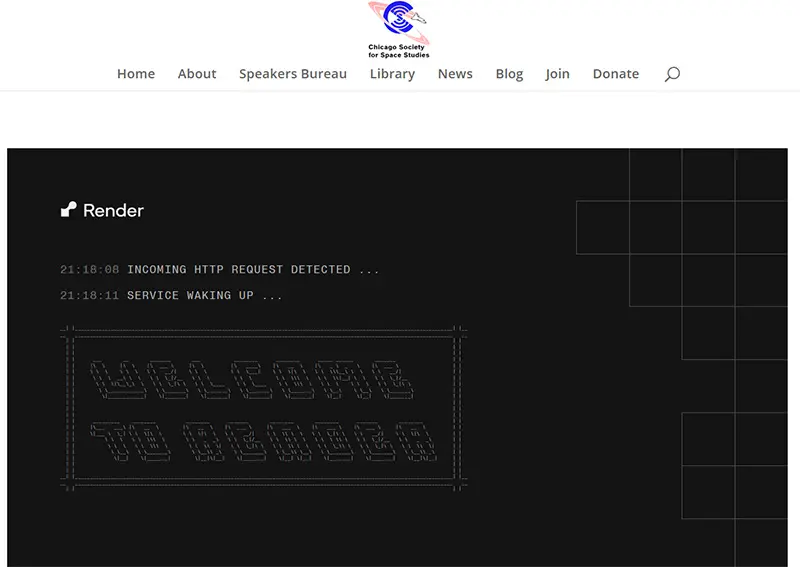
Image 2: The Space Station Design Cost Simulator Web App Starting Up
Please be patient while the program is loading. Loading is complete once the web app’s screen area is like that shown in Image 1.
2) The Program’s Default Screen Display
If you are accessing the application from a desktop or a laptop and have your browser at full screen width, you will see the complete application which consists of the sidebar for user input and the main dashboard for displaying the results of the simulation as shown in Image 1 above.
If you are on a mobile device or are using a narrow screen width, the user input sidebar will be hidden by default and only the dashboard will display. To open the sidebar, click on the gray double arrows that are shown inside the red circle in the Image 3 below.
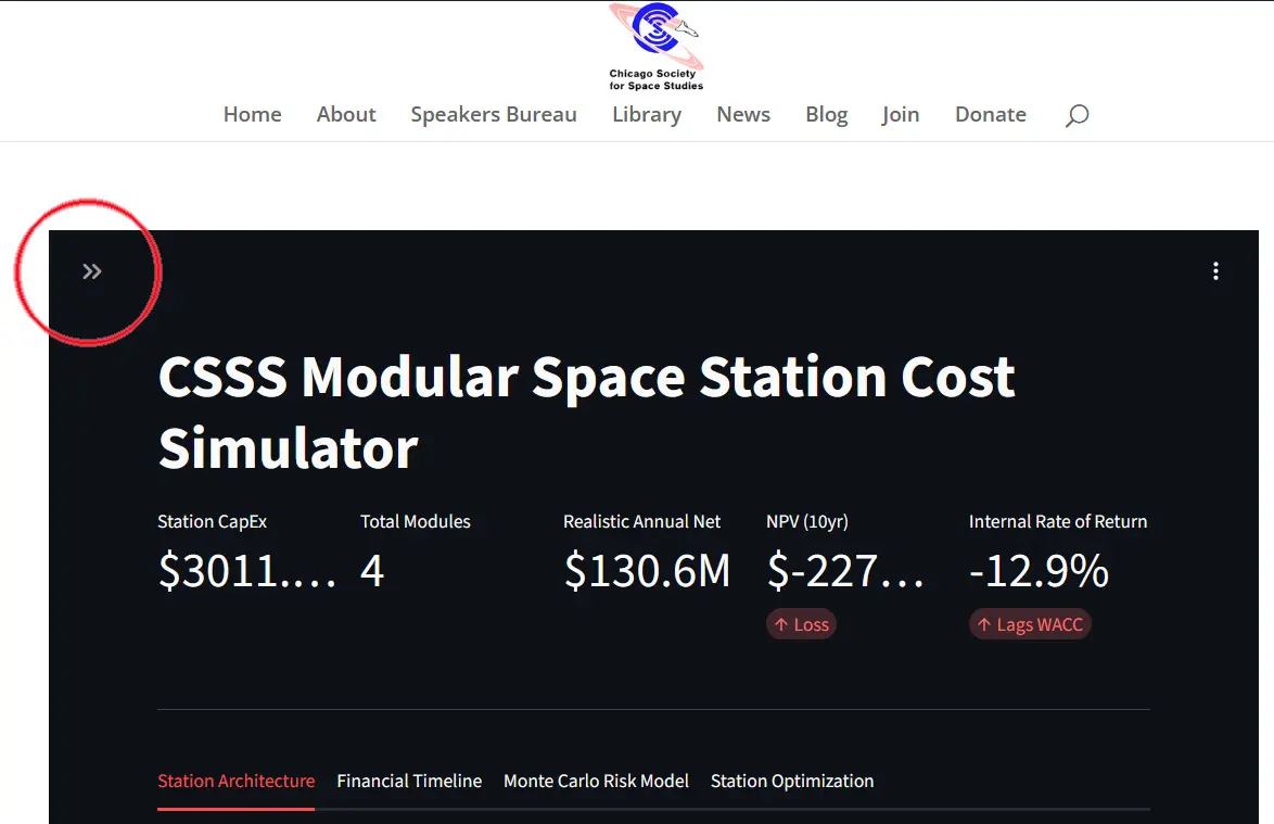
Image 3: Space Station Simulator Screenshot with User Input Sidebar Collapsed
To close the sidebar, click on the gray double arrows that appear in the top right corner of the sidebar as shown in Image 4. Note that these arrows may be hidden from view but will become visible when you move your mouse over the sidebar.
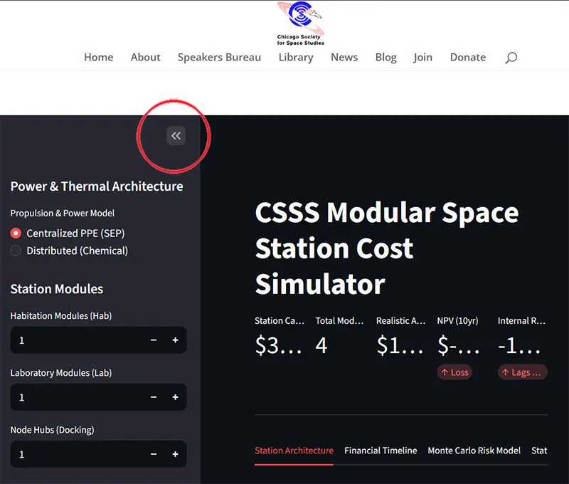
Image 4: How To Collapse the User Input Sidebar
3) Start the Simulation
Before proceeding to read the rest of this user guide, you may find it useful to start the simulation now and familiarize yourself with its layout and controls. Clicking the button below will start the program running in a new browser tab so that you can return to this documentation page without having to exit your simulation.
User Inputs
A suite of parameters is provided so that you can customize the design of your space station. All of these user inputs are located in the program’s left sidebar. They are grouped into five sections. Be aware that as you change each input value, the simulation is automatically updated to reflect that change.
Power & Thermal Architecture Input Section
The Power & Thermal Architecture Input Section is where you will select whether you want to use a single Power & Propulsion Element (PPE) module that uses Solar Electric Propulsion (SEP) for station keeping or will rely on standard chemical thrusters using storable propellant.
The impact of this choice on your space station’s economics is best seen after you have made the rest of your design selections.
Input |
Options / Range |
Description |
Propulsion & Power Model |
Centralized PPE (SEP) or |
Selects the station’s primary power and propulsion architecture. This choice propagates through every calculation. Mass budgets, costs, propellant type, and ISP values all change depending on the selection. |
Station Modules Input Section
This section of selections is self-explanatory. In addition to these three space station module settings, there is also the Power & Propulsion Element (PPE) module whose presence is determined based on whether or not you selected the Centralized PPE (SEP) or Distributed (Chemical) option for the Propulsion & Power Model input. A dedicated module is created if you selected the Centralized PPE (SEP) option since the PPE houses the solar arrays and SEP thrusters.
Input |
Range / Default |
Description |
Habitation Modules (Hab) |
0–10, default 1 |
Number of crew living quarters modules. Each Hab houses the number of crew and tourists set by the Crew parameters below. Volume and mass scale with crew count and the Habitability Standard slider. |
Laboratory Modules (Lab) |
0–10, default 1 |
Number of science/research modules. Each Lab contains 12 experiment racks and no crew berths. Labs are the primary revenue-generating assets through rack-lease income. |
Node Hubs (Docking) |
0–5, default 1 |
The number of connecting node modules. Nodes provide docking ports and passageways between the other modules. Their count is independent here but the Optimization tab auto-calculates nodes as ceil((Habs + Labs) / 3). |
Crew & Tourism Parameters Input Section
This section of selections is also self-explanatory. It is important to note that in this simulation it is assumed that there will be only one tourist flight per year to the space station. This means that the number of Tourists per Hab that you select will all be on the same flight and occupying the space station at the same time. This simulation also over-engineers the station by assuming that all crew and tourists inhabit the space station for a full year.
Input |
Range / Default |
Description |
Crew Members per Hab |
1–6, default 4 |
The number of professional astronauts assigned to each Hab module. This value drives Hab volume based on the user-specified Habitability Standard. |
Tourists per Hab |
0–8, default 3 |
The number of paying space tourists per Hab module. Note: this simulation assumes one tourism flight per year and full year occupancy. |
Habitability Standard (m³ Per Crew) |
8.0–40.0, default 20.0 |
The personal living volume allocated per person in each Hab module, in cubic meters. A setting of 8.0 m³ represents a survival-level minimum; 20.0 m³ is the nominal ISS-standard; 40.0 m³ is deemed a luxury level. This value has a large impact on module volume, hull mass, DDT&E, manufacturing cost, and launch cost. |
Logistics & Market Input Section
This section makes it easy to see how the selection of a launch vehicle impacts the deployment and operational costs of a space station. The ability to set the Water Recycling percentage is useful and impacts the frequency of resupply missions.
Input |
Range / Default |
Description |
Launch Vehicle |
Starship or |
Selects the rocket used to launch all station hardware. This choice sets two key parameters: the fairing volume limit (which caps maximum module size) and the cost per kilogram to orbit (which drives launch CapEx and annual OpEx for propellant and consumable resupply). If the largest module volume exceeds the selected vehicle’s fairing, a red FAIRING FAILURE error halts execution. |
Water Recycling % |
0–99%, default 90% |
The fraction of wastewater reclaimed and reused aboard the station. A higher recycling rate directly reduces the daily water mass that must be launched from Earth, lowering annual logistics OpEx. At 90% only 10% of the base water demand of 3.5 kg/person/day must be resupplied by launch. |
Economic Measures Input Section
Input |
Range / Default |
Description |
Manufacturing Learning Curve (%) |
70–100%,
|
The Wright’s Law learning rate applied to module manufacturing. At 85%, each time cumulative production doubles the per-unit cost falls to 85% of its prior value. A rate of 100% means no learning (costs stay flat). A rate of 70% represents rapid cost reduction with scale. This affects all module manufacturing costs but not DDT&E or power/thermal system costs. |
Market Capacity Factor (Utilization %) |
40–100%,
|
A discount applied to the theoretical maximum annual revenue. It accounts for vacant tourist seats, idle rack time, scheduling gaps, and market demand uncertainty. At 75%, the station earns 75% of what it theoretically could if every seat and rack were always sold and occupied. |
Tourist Ticket Price ($M) |
Default $55.0M |
The price per tourist seat per flight rotation, in millions of dollars. This is the primary revenue lever for the tourism income stream. Multiplied by total tourist seats (num_habs × tourists_per_hab) to compute the maximum annual tourism revenue before the capacity factor is applied. |
Financial Assumptions Input Section
The Discount rate (Weighted Average Cost of Capital or WACC) is used to discount future cash flows back to their present value in the Net Present Value (NPV) formula. Together, they determine if an investment will generate enough revenue to satisfy the capital market. Ideally we want to see a Net Present Value for the project, as opposed to a negative value which means that the project is operating at a loss.
The Project Lifespan is also critical in that the more years for which the station can generate revenue, the more likely it is to be profitable since there are more years available in which to recover the initial capital expenses.
Input |
Range / Default |
Description |
Discount Rate (WACC %) |
5–25%,
|
The Weighted Average Cost of Capital used to discount future cash flows back to present value for the NPV calculation. A higher WACC reflects higher investor risk expectations and reduces NPV. The IRR metric is compared against this rate to determine whether the project ‘beats’ the cost of capital. |
Project Lifespan (Years) |
5–20
years, |
The number of operational years over which the station generates revenue and incurs operating expenses. This window defines the cash flow series used for the NPV and IRR. It also sets the x-axis range on the Financial Timeline chart. |
Space Station Simulation Program Outputs
The program’s dashboard is divided into a top summary metric bar and four analysis tabs. A PDF report download is available from the sidebar.
The simulation output is divided into 5 sections. The top-row section displays at all times. The four specialized tabs are:
Station Architecture
Financial Timeline
Monte Carlo Risk Model
Station Optimization
For reference, see IMAGE 1: space-station-simulation-main-screen-layout.webp
The data for the Station Architecture tab is displayed by default. To display the results for one of the other three tabs, click on the tab’s name. When active, the color of the name will change to red.
Top-Row Summary Metrics
There are five metrics displayed side-by-side across the full width of the main panel:
For the Value Shown column, ‘9’ is a placeholder for whatever the numeric value will be.
Metric Card |
Value Shown |
Delta Indicator |
Meaning |
Station CapEx |
$9.9M |
None |
Total non-recurring + launch costs to build and deploy the station. |
Total Modules |
9 |
None |
The total number of Habs, Labs, Nodes, and PPE modules in the current design. |
Realistic Annual Net |
$9.9M |
None |
Annual revenue minus annual operating expenses (OpEx) after the capacity factor discount. |
NPV (N yr) |
$9.9M |
‘Profitable’ / ‘Loss’ |
Discounted net present value over the user’s lifespan. An indicator will appear under the number identifying a profit or a loss. |
Internal Rate of Return |
9.9% |
‘Beats WACC’ / ‘Lags WACC’ |
IRR vs. the discount rate, aka WACC. .The indicator under the value will be green if IRR exceeds WACC and Red if IRR is less than WACC. |
Station Architecture Tab
This tab consists of a two-column layout with text summaries of key values:
Left Column: Financial Architecture |
Right Column: Operational Physics |
Total R&D (DDT&E): one-time R&D cost in millions of dollars |
Total System Power Demand: Total kilowatts (kW) of electricity needed |
Module Manufacturing (Wright’s Law Applies): modules cost with learning curve in millions of dollars |
Combined Atmospheric Drag Area: The total area of the space station in square meters (m²) used for calculating drag |
Maximum Potential Revenue: total revenue from experiment racks and tourists in millions of dollars per year |
Annual Re-boost Propellant: The total mass of propellant in kilograms (kg) required to maintain the space station in its orbit of 415km |
Risk-Adjusted Revenue (75% Cap Factor): Revenue in millions of dollars per year based on the capacity factor |
|
Financial Timeline Tab
The Financial Timelins is an interactive line chart that shows the cumulative space station net value over the project’s lifespan. Year 0 starts at a negative value that represents the total capital expenditures to begin operation − the initial investment. Each subsequent year adds that year’s net annual income to the chart. A red dashed horizontal line marks the break-even threshold of $0.00. The point where the blue line crosses above zero is the payback period. Image 5 below shows the default financial timeline chart.
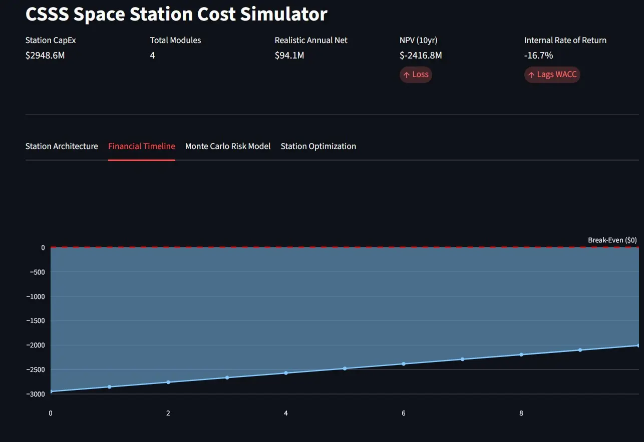
Image 5: Space Station Simulator Financial Timeline Graph
Image 6 below shows a space station configuration which is profitable.
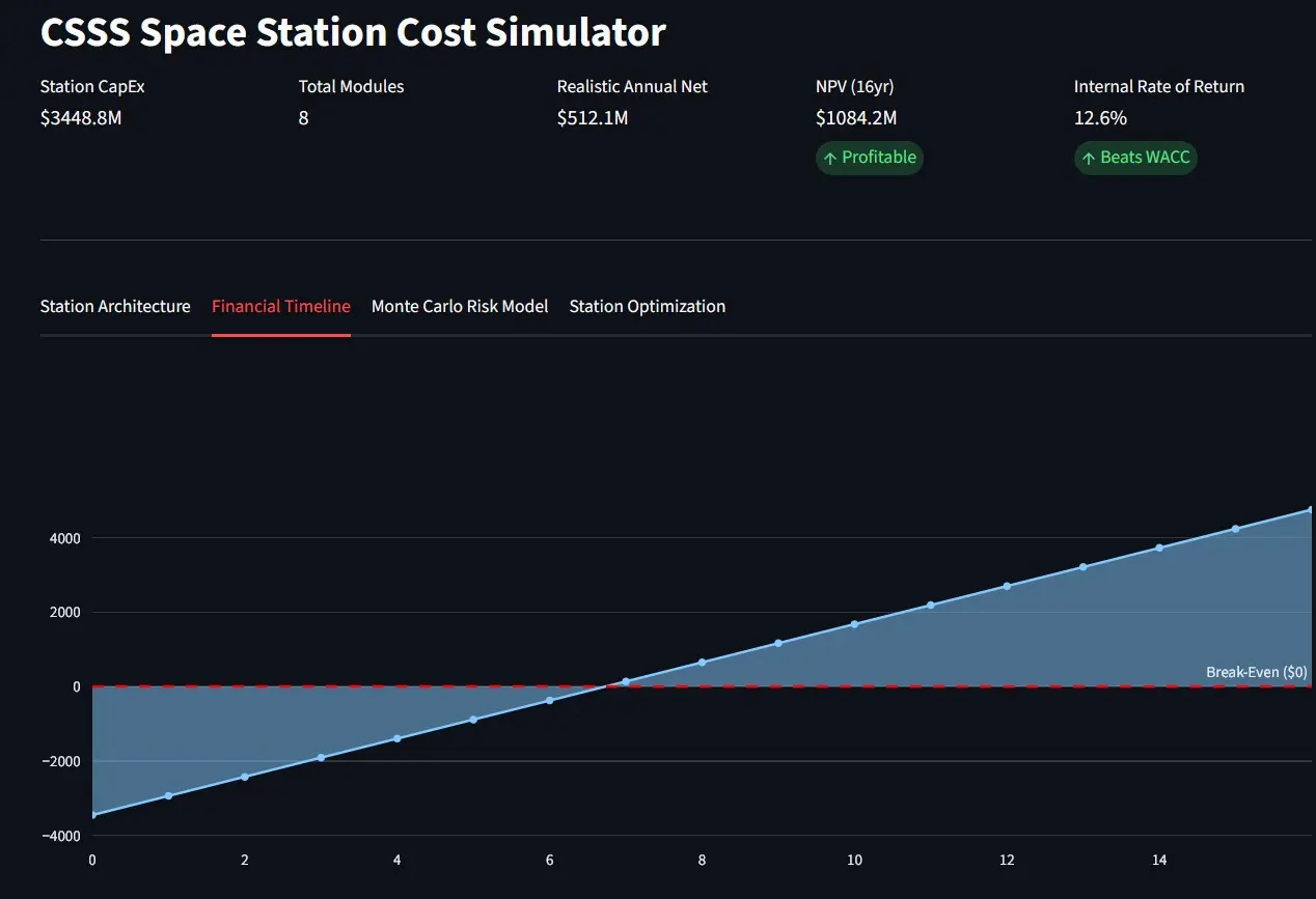
Image 6: Space Station Simulator Financial Timeline Graph Showing a Profit
Monte Carlo Risk Model Tab
When you activate the Monte Carlo Risk Model tab, your screen will display as shown in Image 7.
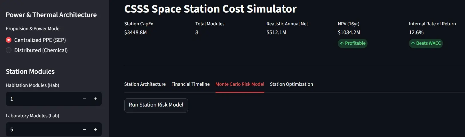
Image 7: Monte Carlo Risk Model Report Initial State
The Monte Carlo Risk Model is unique in that it must be manually started by the user by clicking the Run Station Risk Model button. Upon clicking the Run Station Risk Model button, the simulator will create 10,000 variations of the space station model and produce a chart that summarizes the results. The focus of the simulation is on variations to the financial aspects of the space station business and serves as an introduction to a financial risk analysis technique. Image 8 is a representation of one such set of 10,000 financial simulations.
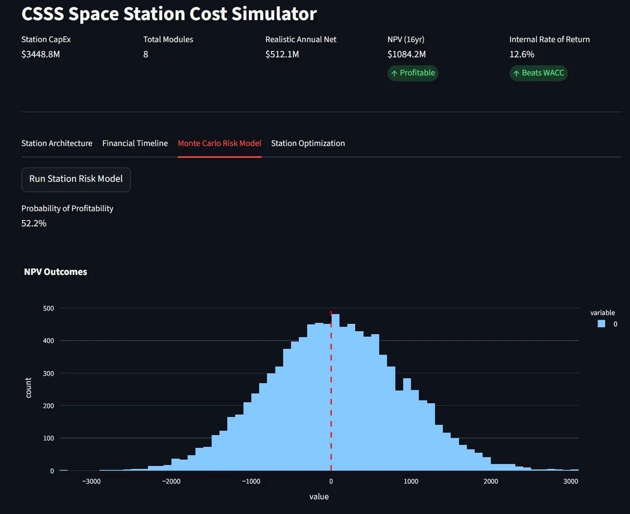
Image 8: Monte Carlo Risk Model Report Chart Output
Each of the 10,000 runs represents a set of financial variants in which:
Capital Expenditures (CapEx) are sampled from a uniform range of 1.1x to 1.5x the base value
Operating Expenses (OpEx) are sampled from a normal distribution with 10% volatility.
Launch costs are sampled from a distribution ranging from 0.8x to 2.0x of the launch list price
Annual Revenues are sampled from a normal distribution with 15% volatility
Each of these 10,000 simulations produces its own Net Present Value (NPV) for that set of financial conditions. This type of risk analysis is important since nothing about the future is known for certain. Launch costs can rise, revenues can fall short, the capital expenditures may be greater than planned. Testing for a range of possibilities offers investors and the owners a better perspective of the degree of financial risk associated with the project.
The graph that is produced is a histogram of the simulated NPV values. The chart distributes the NPVs into 100 bins titled `NPV Outcomes`. The red vertical line at zero marks the break-even point. Values to the right of that line represent profitable scenarios while values to the left are loss scenarios.
How to read the Monte Carlo Chart
The Monte Carlo graph charts NPV dollar amounts (Y axis) and the number of time that value was produced (X axis). A histogram that is concentrated to the right of the red vertical line (the zero point) means that the project is profitable under the model’s uncertainty assumptions. A histogram that is centered near zero means the project is borderline: profitability and unprofitability are equally likely. A histogram that lies mostly left of zero means the project is likely unprofitable. A Probability of Profitability metric is provided (on the left side and above the chart) to show the percentage of simulated NPVs that were greater than zero. The larger this percentage is, the more confident you can be that your space station will be profitable. By modeling a set of probabilistic outcomes rather than a singular, deterministic prediction, the simulator allows us to have a better understanding of the projects financial risks.
The following table summarizes the variations that are made for each of the 10,000 simulations that are run.
Variable |
Distribution & Parameters |
CapEx |
A uniform distribution of (base × 1.1) to (base × 1.5) on the assumption that cost overruns are far more likely than cost underruns. |
Launch Cost |
An asymmetric distribution with a minimum of 0.8 and a maximum of 2.0 times the stated launch cost. |
Annual Revenue |
A normal distribution with a standard deviation of 15%. |
Annual OpEx |
A normal distribution with a standard deviation of 10%. |
Station Optimization Tab
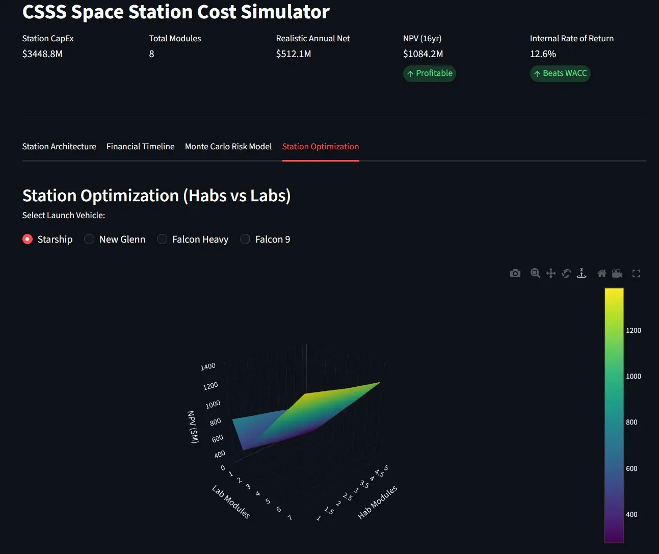
Image 9: Station Optimization Report Tab
The purpose of the Station Optimization report is to render an interactive optimization grid that produces a 3-D surface plot of Net Present Value (NPV) vs. Hab modules vs. Lab modules for the launch vehicle that is selected at the top of the chart. The importance of this graph is that it illustrates the relationship between Net Present Value (NPV) on the Z axis, the number of Hab modules on the X axis, and the number of Lab modules on the Y axis. This graph can be rotated and zoomed using the controls provided. For the precise number at a location on the graph’s surface, placing your mouse over that data point on the graph will cause a pop-up to be displayed that shows the exact values for that location, as shown in Image 10 below.
IMAGE 10: space-station-simulation-output-detail-view.webp
The high points or peaks in the graph represent the best combination of hab and lab modules. You will note that the Net Present Values in the Image 10 graph are all negative, meaning the current space station design combined with the chosen launch vehicle has no shot at being profitable. This graphic visualization illustrates a lesson in systems engineering: that optimal designs only emerge through quantitative analysis of competing constraints.
PDF Executive Report
Users have the option to save their simulation as an executive report to a PDF file. To initiate the creation of the report, click the Download Report (PDF) located at the bottom of the user input sidebar.
The report has three sections:
1. Station Architecture
2. Operational Physics & Constraints
3. Financial Projections & Economics
The report consists of the following fields.
1. Station Architecture
Field Name |
Field Contents |
Launch Vehicle |
The launch vehicle selected by the user |
Total Modules |
The total number of modules for the space station |
Habitation Modules |
The number of habitation modules |
Laboratory Modules |
The number of laboratory modules |
Node Modules |
The number of node modules |
Power/Propulsion Element |
Reflects the user’s Propulsion & Power Model choice |
Total Crew |
The total number of station crew members |
Total Tourists |
The total number of tourists |
2. Operational Physics & Constraints
Field Name |
Field Contents |
System Power Demand |
The total energy in kilowatts the station requires |
Active Radiator Area |
The total area in square meters of the station’s radiators |
Atmospheric Drag Area |
The total area in square meters of the station’s atmoshperic drag |
Annual Re-boost Fuel |
The total amount of propellant in kilograms needed for the station to maintain its orbit |
3. Financial Projections & Economics
Field Name |
Field Contents |
Total CapEx (R&D+Mfg+Launch) |
The total capital expenditures needed to design, build, and launch the space station given in millions of dollars |
Risk-Adjusted Annual Revenue |
Annual revenue in millions of dollars based on maximum revenue multiplied by the user specified Market Capacity Factor |
Annual OpEx |
Annual operating expenses in millions of dollars |
Project Lifespan |
User specified space station operational life in years |
Discount Rate (WACC) |
User specified Weighted Average Cost of Capital (WACC) |
Simulator Limitations
This space station design simulator has a number of limitations and restrictions that limit the realism of the simulation. These limitations are meant to balance simplicity against complexity in order to make the simulation more accessible. These limitations also serve to minimize the program’s impact on server resources – which have strict CPU, memory, and bandwidth limits.
Some of the simplifications are:
No external payloads option, thus foregoing a possible revenue stream
Pricing for the station’s experiment racks is static and controlled by the user’s Market Capacity Factor selection
Assumes equal occupancy per hab module (equal density housing vs high/low density housing). This is in part a consequence of the cost savings of being able to mass produce hab modules versus manufacturing ‘bespoke’ hab modules one at a time.
Assumes a fixed minimum crew-to-tourists ratio.
Assumes that there will be only one tourist flight per year to the space station.
Assumes all nodes are equally sized and configured.
Relies on static Cost Estimating Relationships (CER) to calculate DDTE costs.
Space Station Design Challenges
Following are some questions you may ask yourself while designing your space station within the framework of the simulation:
- Space station sizing is done based on peak occupancy (crew + tourists) so what impact does my selection of crew size and habitability standards have on my station’s total cost?
- Experiment rack revenue is assigned a fixed dollar value per rack and is tied to my Market Capacity Factor selection but what will be the actual revenue per rack?
- Kilowatt usage is assumed to be the same for crew and tourists. How true will that be?
- What is the best combination of crew and tourists?
- Is the default tourist ticket price of $55 million realistic? What happens to profitability as I change the number of tourists and raise/lower the ticket price?
- How big of an impact does the Habitability Standard have on capital expenditures (CaPeX)?
- What is the optimal balance of hab to lab modules?
- What happens as I change the Manufacturing Learning Curve and increase the number of modules?
Relevant System Configuration Constants
The program uses a number of preset (hard-coded) constant values that are used as a part of the calculation processes. For reference purposes, the most relevant constants for users are listed here in alphabetical order.
Variable Name |
Value |
Variable Purpose |
| ATMOS_DENSITY_KG_M3 |
1×10⁻¹² kg/m³ |
The atmospheric density at LEO (~400 km) used in calculating aerodynamic drag. |
| BASE_SYSTEM_KW |
10.0 kW |
Minimum station-wide power load for avionics, communications, and environmental control, etc. This value is separate from crew and experiment consumption. |
| CHEM_COST_PER_KW_M |
$0.75M/kW |
Capital cost of the chemical power system per kilowatt. |
| CHEM_ISP |
300 s |
Specific impulse of chemical thrusters which have much lower ISP than SEP. |
| CHEM_MASS_PER_KW |
15.0 kg/kW |
Mass of a chemical/battery power system per kilowatt. Heavier than SEP due to battery storage requirements. |
| CREW_BASE_DAILY_KG |
2.9 kg/person/day |
Daily mass of non-water consumables per person: food, oxygen, hygiene supplies, and waste bags. |
| CREW_WATER_DAILY_KG |
3.5 kg/person/day |
Daily water consumption per person before recycling. The water_recycle_rate slider reduces the fraction that must be resupplied from Earth. |
| DDTE_BASE_MILLIONS |
15.0 $M |
Scale factor (in millions of dollars) in the DDT&E Cost Estimating Relationship (CER). |
| DDTE_EFFICIENCY_MULT |
0.85 |
A global efficiency factor applied to all DDT&E estimates. Represents expected design reuse and efficiency compared to a fully new, bespoke spacecraft program. |
| DDTE_MASS_EXP |
0.55 |
Exponent in the DDT&E cost estimating relationship (CER) – it reflects spacecraft development cost data where costs scale with mass. |
| DRAG_COEFFICIENT |
2.2 |
A dimensionless drag coefficient that is a representative value for spacecraft structures. |
| GROUND_OPS_OVERHEAD_RATE |
0.10 |
Ground operations cost expressed as 10% of realized annual revenue. It covers mission control, data handling, and administrative overhead. |
| HAB_DDTE_MULT |
1.0 |
DDT&E multiplier for Hab modules |
| HAB_OVERHEAD_M3 |
10.0 m³ |
Fixed structural overhead volume in a Hab module (corridor, airlock, walls, etc.). |
| HAB_RACK_CAPACITY |
2.0 racks |
Number of equipment racks in each Hab module (e.g., for stowage or small experiments). |
| HULL_SCALING_COEFF |
95.0 |
Coefficient in the hull mass power-law calibrated so that a typical ISS module yields a plausible structural mass. |
| HULL_SCALING_EXP |
0.667 |
Exponent in the hull mass formula. A 2/3 exponent reflects the surface-area-to-volume relationship of pressure vessel mass where doubling volume increases hull mass by a factor of ~1.59, not 2.0. |
| KW_PER_CREW |
2.5 kW |
Power demand per crew/tourist member that covers life-support, lighting, personal equipment, etc. |
| KW_PER_RACK |
1.5 kW |
The average power draw per equipment rack. |
| LAB_CREW_CAPACITY |
0.0 crew |
Set to 0 to reflect that a Lab module will not contain any crew quarters. |
| LAB_DDTE_MULT |
0.8 |
DDT&E multiplier for Lab modules. Labs are 20% cheaper to develop than Habs due to less human-factors engineering complexity. |
| LAB_OVERHEAD_M3 |
20.0 m³ |
Fixed structural overhead volume in a Lab module (larger than Hab due to rack bay structure). |
| LAB_RACK_CAPACITY |
12.0 racks |
Number of experiment racks in each Lab module. This is the primary research capacity driver. |
| MFG_COST_PER_KG |
$15,000/kg |
Manufacturing cost rate for the first production unit of each module type. Multiplied by hull mass to get first-unit cost. |
| NODE_DDTE_MULT |
0.5 |
DDT&E multiplier for Node hubs. Structurally simple with no unique systems. |
| NODE_RATIO_DIVISOR |
3.0 |
Used in the Optimization tab to auto-calculate node count with one node per three hab/lab modules. |
| NODE_VOL_M3 |
35.0 m³ |
Fixed total internal volume of a Node hub module. |
| ORBITAL_VELOCITY_M_S |
7,660 m/s |
Mean orbital velocity at LEO based on an orbit of 415km. |
| PPE_DDTE_MULT |
1.5 |
DDT&E multiplier for the PPE module. Set to be 50% more expensive to develop than a Hab due to complex propulsion and power integration. |
| PPE_VOL_M3 |
50.0 m³ |
Fixed total internal volume for the Power & Propulsion Element (PPE) module. |
| RACK_MASS_KG |
800 kg |
Mass of a single International Standard Payload Rack (ISPR). Lab and Hab racks are all assumed to be this mass. |
| RACK_REV_PER_YEAR_M |
$2.5M/rack/yr |
Annual lease revenue per experiment rack. Represents income from government agencies or commercial researchers paying for access to microgravity research facilities. |
| RACK_VOL_M3 |
1.5 m³ |
Volume consumed by one equipment rack inside a module. |
| RAD_AREA_PER_KW |
3.5 m²/kW |
Radiator panel area required per kilowatt of thermal rejection. Contributes to the station’s total drag area. |
| SEP_COST_PER_KW_M |
$1.2M/kW |
Capital cost of the Solar Electric Power (SEP) system per kilowatt. Higher unit cost than chemical, but offset by lower propellant OpEx. |
| SEP_GLIDER_EFFICIENCY |
0.70 |
Effective drag-area efficiency of SEP solar arrays. SEP arrays are actively pointed, so only 70% of their area is counted as drag-contributing at any given time. |
| SEP_ISP |
2,000 s |
Specific impulse of the SEP ion/Hall thruster. Very high Isp means very low propellant mass consumption per unit of delta-v. |
| SEP_MASS_PER_KW |
12.0 kg/kW |
Mass of the SEP power system (solar arrays + power electronics) per kilowatt of capacity. |
| SEP_PROPELLANT_PRICE_KG |
$5,000/kg |
Cost of xenon propellant per kilogram. This is added to the launch cost per kg when computing annual propellant resupply OpEx for SEP stations. |
| SOLAR_AREA_PER_KW |
6.0 m²/kW |
Solar array area required per kilowatt of generated power. Contributes to station’s total drag. |
| THERMAL_COST_PER_KW_M |
$2.5M/kW |
Capital cost of the thermal rejection system per kilowatt. The most expensive system on a per-kW basis. |
| THERMAL_MASS_PER_KW |
25.0 kg/kW |
Mass of the thermal rejection system (heat pipes, radiators) per kilowatt of heat to be rejected. |
Launch Vehicle Constants
The Launch Vehicle Constants consist of the Fairing Volume and Cost per Kilogram (kg) values for each of the available launch vehicles. Fairing Volume is the constraint that limits the maximum module size. Cost per kilogram is the launch cost applied to all mass lifted to orbit with initial station dry mass being captured as a capital expenditure (CapEx) and the annual propellant and consumables resupply being captured as an operating expense (OpEx).
Launch Vehicle |
Fairing Volume (m³) |
Cost per kg ($) to LEO |
Starship |
1,000.0 |
$500 |
New Glenn |
450.0 |
$2,200 |
Falcon Heavy |
145.0 |
$1,500 |
Falcon 9 |
145.0 |
$2,720 |
Error Conditions & Validation
The error conditions listed here are internal to the simulation and are generated when some calculation or user input fails to meet the simulation’s criteria. Any other errors that may occur will be associated with a problem with one of the servers associated with this application.
Condition |
Trigger |
Behavior |
Crew to Tourists ratio out of bounds |
There are more than 2x as many tourists as crew. |
Red sidebar error banner + st.stop(). The app stops until the user changes either the number of crew or tourists. |
Module exceeds fairing |
A module is larger than the fairing limit of the launch vehicle. |
Red main-panel error with exact volumes shown. The user needs to either change launch vehicles or the parameters associated with module sizing. |
IRR computation fails |
Calculating the IRR returns an error. |
The program continues but with the IRR is set to 0%. |
No viable optimization configuration |
All Hab/Lab combos fail the fairing check for a rocket |
Red error message ‘No viable configurations found’ in Tab 4. |
Future Developments
At this time, the following modifications are being considered for future versions of the simulator:
Dedicated Tourist Module
Multiple Tourist Flights Per Year
User control of tourist stay duration
External Payloads Capability
A major consideration with respect to added simulation complexity is that any future additions to the simulator will need to operate within hosting restrictions (CPU, memory, bandwidth) imposed on the application by the hosting agreement.
Author Biography: Jim Plaxco is President of Chicago Society for Space Studies, a member of the CSSS Speakers Bureau, and a National Space Society Space Ambassador. Jim was elected to the NSS Board of Directors for the third time in 2024 and has previously held the positions of NSS Vice President for Chapters, NSS Director of Information Systems, Vice President of Planetary Studies Foundation, and President of Northern Illinois Space Advocacy.